Quick tip - How to format your data with one click?

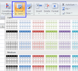
Excel 2007 gives you an option to format your data in one click using the Format as Table option available on the ribbon.

Lets take an example - Suppose this is your data

To quickly format select your data and go to Styles group of the Home tab in the ribbon then click on Format as Table dropdown and select the appropriate format.

As you selected the data there will be no need to change anything in the Format Table dialog box, so simply click Ok.

And that is it........

Inserting Comments with your name

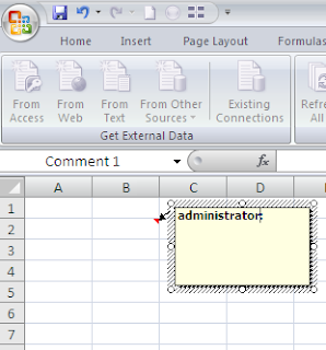
Have you ever faced a situation when you insert a comments and it shows either your email or administrator in the comment box?

Something like this

Now you are left with two options - one leave it as it is (which does not look nice at all to the people who are using the file) or to change it. You can change it everytime by simply overwriting it.

There is another option using which you can change it forever. Follow these steps to change it permanatly in your excel files.

Step 1 : Go to Excel Options

Step 2 : On the popular tab change the user name & click ok.

All your Insert Comment commands from now on will have the changed user name.

Vlookup Example

Vlookup searches for a value in the leftmost column of a table, and then returns a value in the same row from a column you specify in the table. Use VLOOKUP instead of HLOOKUP when your comparison values are located in a column to the left of the data you want to find.

The V in VLOOKUP stands for "Vertical."

Syntax

VLOOKUP(lookup_value,table_array,col_index_num,range_lookup)

Lookup_value    is the value to be found in the first column of the array. Lookup_value can be a value, a reference, or a text string.

Table_array    is the table of information in which data is looked up. Use a reference to a range or a range name, such as Database or List.

Col_index_num    is the column number in table_array from which the matching value must be returned. A col_index_num of 1 returns the value in the first column in table_array; a col_index_num of 2 returns the value in the second column in table_array, and so on. If col_index_num is less than 1, VLOOKUP returns the #VALUE! error value; if col_index_num is greater than the number of columns in table_array, VLOOKUP returns the #REF! error value.

Range_lookup    is a logical value that specifies whether you want VLOOKUP to find an exact match or an approximate match. If TRUE or omitted, an approximate match is returned. In other words, if an exact match is not found, the next largest value that is less than lookup_value is returned. If FALSE, VLOOKUP will find an exact match. If one is not found, the error value #N/A is returned.

Example

	A	B	C	D
1	Density	Viscosity	Temperature	Vlookup
2	0.457	3.55	500	=VLOOKUP(A2,A2:C7,2,TRUE)
3	0.525	3.25	400
4	0.616	2.93	300
5	0.675	2.75	250
6	0.746	2.57	200
7	0.835	2.38	150

Looks up 0.457 in column A, and returns the value from column B in the same row. This will result 3.55

Countif Function Example

It Counts the number of cells within a range that meet the given criteria.

Syntax

COUNTIF(range,criteria)

Range          is the range of cells from which you want to count cells.

A Criteria       is the criteria in the form of a number, expression, or text that defines which cells will be counted. For example, criteria can be expressed as 32, "32", ">32", "apples".

Example

	A	B	D
1	Data	Data	Count If
2	apples	32	=COUNTIF(A2:A5,"apples”)
3	oranges	54
4	peaches	75
5	apples	86

Counts the number of apples written as text in the range A2 to A5, and returns the count. This will result 2.

MS Excel – Shortcut Keys

Key Description
CTRL+(	Unhides any hidden rows within the selection.
CTRL+)	Unhides any hidden columns within the selection.
CTRL+&	Applies the outline border to the selected cells.
CTRL+_	Removes the outline border from the selected cells.
CTRL+~	Applies the General number format.
CTRL+$	Applies the Currency format with two decimal places (negative numbers in parentheses).
CTRL+%	Applies the Percentage format with no decimal places.
CTRL+^	Applies the Exponential number format with two decimal places.
CTRL+#	Applies the Date format with the day, month, and year.
CTRL+@	Applies the Time format with the hour and minute, and AM or PM.
CTRL+!	Applies the Number format with two decimal places, thousands separator, and minus sign (-) for negative values.
CTRL+-	Displays the Delete dialog box to delete the selected cells.
CTRL+*	Selects the current region around the active cell (the data area enclosed by blank rows and blank columns). In a PivotTable, it selects the entire PivotTable report.
CTRL+:	Enters the current time.
CTRL+;	Enters the current date.
CTRL+`	Alternates between displaying cell values and displaying formulas in the worksheet.
CTRL+'	Copies a formula from the cell above the active cell into the cell or the Formula Bar.
CTRL+"	Copies the value from the cell above the active cell into the cell or the Formula Bar.
CTRL++	Displays the Insert dialog box to insert blank cells.
CTRL+1	Displays the Format Cells dialog box.
CTRL+2	Applies or removes bold formatting.
CTRL+3	Applies or removes italic formatting.
CTRL+4	Applies or removes underlining.
CTRL+5	Applies or removes strikethrough.
CTRL+6	Alternates between hiding objects, displaying objects, and displaying placeholders for objects.
CTRL+7	Displays or hides the Standard toolbar.
CTRL+8	Displays or hides the outline symbols.
CTRL+9	Hides the selected rows.
CTRL+0	Hides the selected columns.
CTRL+A	Selects the entire worksheet. If the worksheet contains data, CTRL+A selects the current region. Pressing CTRL+A a second time selects the entire worksheet. When the insertion point is to the right of a function name in a formula, displays the Function Arguments dialog box. CTRL+SHIFT+A inserts the argument names and parentheses when the insertion point is to the right of a function name in a formula.
CTRL+B	Applies or removes bold formatting.
CTRL+C	Copies the selected cells. CTRL+C followed by another CTRL+C displays the Microsoft Office Clipboard.
CTRL+D	Uses the Fill Down command to copy the contents and format of the topmost cell of a selected range into the cells below.
CTRL+F	Displays the Find dialog box. SHIFT+F5 also displays this dialog box, while SHIFT+F4 repeats the last Find action.
CTRL+G	Displays the Go To dialog box. F5 also displays this dialog box.
CTRL+H	Displays the Find and Replace dialog box.
CTRL+I	Applies or removes italic formatting.
CTRL+K	Displays the Insert Hyperlink dialog box for new hyperlinks or the Edit Hyperlink dialog box for selected existing hyperlinks.
CTRL+L	Displays the Create List dialog box.
CTRL+N	Creates a new, blank file.
CTRL+O	Displays the Open dialog box to open or find a file. CTRL+SHIFT+O selects all cells that contain comments.
CTRL+P	Displays the Print dialog box.
CTRL+R	Uses the Fill Right command to copy the contents and format of the leftmost cell of a selected range into the cells to the right.
CTRL+S	Saves the active file with its current file name, location, and file format.
CTRL+U	Applies or removes underlining.
CTRL+V	Inserts the contents of the Clipboard at the insertion point and replaces any selection. Available only after you cut or copied an object, text, or cell contents.
CTRL+W	Closes the selected workbook window.
CTRL+X	Cuts the selected cells.
CTRL+Y	Repeats the last command or action, if possible.
CTRL+Z	Uses the Undo command to reverse the last command or to delete the last entry you typed. CTRL+SHIFT+Z uses the Undo or Redo command to reverse or restore the last automatic correction when AutoCorrect Smart Tags are displayed.

How to get the Developer Tab in the Ribbon

From where do you insert a command button in MS Excel 2007?

The option is available on the Developer tab of the ribbon.

In case the Developer Tab is not appearing in your Excel 2007 ribbon, the option has not been enabled on your machine.

To enable the option, follow these steps:

Click on Excel Options under the Office Button



Once on the Excel Options dialog box check the "Show Developer tab in the ribbon" check box & click Ok.

MS Excel 2007 Save as PDF

Ever wanted to save or export your excel contents to PDF?

In MS Office 2007, you have an Add in which can help to save your Word, PowerPoint or Excel files as PDF.

You can install this add in from this link

http://www.microsoft.com/downloads/details.aspx?FamilyID=4d951911-3e7e-4ae6-b059-a2e79ed87041&displaylang=en

Once installed the feature to save the file as PDF is available under Office Button - Save As - Save as PDF

That is it!!! You can easily save your Excel files as PDF.....