Formula on request

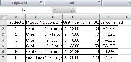
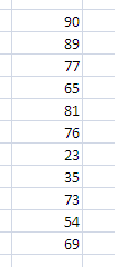
I have been requested a formula, which checks the contents of column A, if it is a number and greater than 0, then number is to be multiplied by 100. If it is a number but is less than 0, the number is to be multiplied by 50. However if it is not a number but some text, text should appear as the result.

Here is it, Have written only single formula, which gives the desired result. Have a look!!!!!

How to add jpeg picture in your comments?

How to add jpeg picture in your comments?

Interesting question??

The answer is, yes, it is possible. Not directly though but you can definitely add a picture to your comments. It can not only make it look different but can also be useful in terms of space utilization.

Want to learn how? Lets have a look at the steps:

1. Add the comment to the cell by right clicking on the cell & by selecting Insert Comment.

2. Select the comment from the red pointed area (the border of the comment) & right click on the selected area. Select Format Comment from the menu.

3. The below dialog box will appear. This is the major point in the steps. Make sure you get a similar dialog box. The best way to find out is, it will have more than one tab. If it shows only one tab, try the step 2 again.

4. Select Color and Lines & then from Fill Color drop down select Fill Effects.

5. From the Fill Effects dialog box select the picture you want to add to the comment by using "Select Picture" button. Once selected, click OK and then OK on the Format Comment dialog box as well.

6.  The end result is a different looking comment :)

You can always try with Katrina Kaif's or Sunny Leone's picture :-P

5 of my most used commands

Thought of listing something which I frequently use. Here is a list of 5 of my most used commands in Excel:

Sort your data using Data - Sort & Filter

Apply Data Validation using Data - Data Tools

Apply Conditional Formatting using Home - Styles

Change the format of text using Home - Font

Create a Pivot table using Insert - Tables

How to get commonly used commands in the Quick Access Toolbar?

Before I write something, please see this:

These are the two commands that I use more than 10 times a day. One is to select Visible cells only and the other one is to Remove Duplicates. I have added these buttons to my Quick Access toolbar so that I do not have to do multiple clicks to perform the operation.

The quick access toolbar can be customized to show any of your commonly used command. To customize it, go to Excel options - Customize. You can select the commands from the left hand side drop down & list box and add them to the toolbar (i.e. the right side listbox).

Hope it will make your task a little quicker!

How to add or remove a background?

Want to show some picture as a watermark to your worksheet?

You can easily add or remove the background with just one click.

To add a background Go to - Page Layout tab of the ribbon

On the Page Layout tab - look for Page Setup group and then click Background. Simply browse to the picture file you want as the background and click Insert after selecting the required file.



The selected picture will be applied. To remove simply click the Delete Background button on the same Page Setup group.



Evaluate formula

Amid this festive, sunday & cricket mood.. lets have another posting....

If you have a lengthy nested formula and you are not sure about the result, it is better to debug and evaluate the formula one step at a time to find out whether the result, which is coming is correct or not.

Now to evaluate this formula step by step follow these steps:

1. Select the cell with the formula, which needs to be evaluated
2. Go to the Formulas tab of the ribbon. On the formulas tab, select evaluate formula from the Formula Auditing group.

3. From the Evaluate formula dialog box, click on evaluate to get the result of the underlined part of the formula. Pressing evaluate again will show the result of the next underlined part of the formula. This process can be repeated till the time the entire formula has been evaluated.

Fill the empty cells below

I am sure you have faced a situation where the data has been copied out of a pivot table, which looks like this

Many a times there is a need that you fill up the empty cells under a section with the same values. Like in the above example you need ABC in row number 2 to 5 and BCD in row number 8 to 11. There are many ways to accomplish this, with Copy - paste, Ctrl + D, Using power utils add in to name a few.

There is a way using formulas and selecting visible cells. To use this way apply the formula in the first empty cell (A3 in our case). The formula should pick up the value from the cell above to it. In our case A3 should contain a formula "=A2".

Follow these steps to fill all the empty cells with the contents which appear once in the section.

1. Copy the cell in which the formula is applied.
2. Apply an auto filter on the same column. Select all the empty cells that come as a result.
3. Filter for the blank cells, press "Ctrl +G". From the Go To dialog box, click on "Special". From the "Go To Special: dialog box select "Visible Cells only" and then click "OK". This will leave only the empty cells which are below the section text.
4. Now paste the formula which you have copied. And all the empty cells will be filled with the section text. 

How to add a ± symbol?

Hello everyone.... I am back... Its been a long time and a lot has happened since June this year. But now I will make sure I am regular contributor :)

Will start with a very small post today. How to add a ± symbol in an excel cell.

Basically this is a symbol which we use in financial & statistical data. To add ± in any cell go to Insert Tab on the ribbon & then click on Symbol from the text group.

From the symbol window, you can select the plus minus symbol. You can find this symbol under the Latin -1 Supplement subset. Once you spot the symbol, select it and then click Insert.

Mini Toolbar

Excel 2007 adds a mini toolbar just above the menu which open when you right click on any cell. This mini toolbar draws useful commands from the Ribbon.

Automatic Calculations

By default an Excel sheet calculates the formula result automatically. This is indeed a great feature with the user only need to worry about the values in the cell, and any change in these values result in changes in the formula result  by its own.

How to remove Data Validations

There are multiple ways to do it and probably the simplest is to copy and paste an empty cell over the cell which contains the data validation. However if you just want to clear the data validation leaving the data & the format intact. Use the Clear All button on the Data Validation dialog box.

Difference between Excel 2003 & Excel 2007

How to remove duplicates

Lets start with the original data which contains the duplicate values. Similar to one shown below

First select the entire data including the header row.

Now go to the Remove Duplicate command which is available on the Data tab of the ribbon

Select the column header from which you want to remove the duplicates, then click ok.

That is it, the duplicates have been removed. You will be shown a message showing how many duplicates have been removed and how many unique values remain.

Quick Tip - How to format Heading rows in one click!

If the Format as Table option formats the entire data and does not suits your requirement to only format the heading row leaving the data intact, follow these steps to quickly format only the heading rows.

E.g. this is your data

Select the heading row and click on the Cell Styles drop down (available on Styles group of the Home tab).

Now select the format which looks presentable to you.

And that is it!!!

Excel 2007 - Filter / Sort by Color!!!!!

Now along with the normal text filtering you can filter by the cell or by the font colors as well. The filter by color option appears in the normal auto filter drop down.

It is as simple as single click....

Similar way even sorting can be done based upon the cell or the font color.

Quick Tip - Traffic Lights in Excel?

Traffic lights, yes the red, yellow & green lights can be created in our own excel as well. Excel 2007 has enhanced feature of conditional formatting, which not only fills the cell's background with a color but can also do a lot more.

Based upon a range of values you can show the Red, Yellow or Green indicators in the cell. To create Traffic light lets take this sample data

Step 1
Select the data and click on the Conditional Formatting drop down from the Styles group of the Home tab

Step 2
Select Icon Sets and then 3 Traffic Lights

If you want to change the conditions, select Manage Rule from the Conditional Formatting drop down.

Select the rule then click on Edit Rule. Change the conditions then click on Ok

You can also check the Show Icon only check box to see only the lights and not the data.

How to change the alignment in the Chart Axis

Many a times when you create a chart the horizontal axis get diagonally aligned by default. This happens to fit the contents in the chart window. If you are wondering what I am talking about, this is how it appears

To change the direction of the text follow these steps

Step 1: - Select the Axis from the chart

Step 2: - Choose the Orientation option on the Alignment group of the Home tab.

Depending upon the option you choose the direction of the text will be changed. In this case it will be rotated upwards like this.