No matter if India lost another one.... here is another excel tip

Cell Function


This function examines a cell and displays information about the contents, position and formatting.

=CELL("TypeOfInfoRequired",CellToTest)
The TypeOfInfoRequired is a text entry which must be surrounded with quotes " ".


The following example uses the =CELL() function as part of a formula which extracts various information

Count functions.... contd....

Continuing where I had left last week on the count functions... let me introduce to you one more count function

Lets have a look at the CountIf function. CountIf alows you to count based on a given criteria. For example you want to count the number of employees with sale above $1000 in the below data

The formula which you can apply will be
=COUNTIF($C$2:$C$9,">1000")

In this formula ">1000", is the criteria, which comprises or the operator greater than. All the relational operators like >, <, <=, >= & <> can be used. These is no need to write equal to, if you want the exact match of 1000 (use "1000" in that case).

Evaluate formula

Amid this festive, sunday & cricket mood.. lets have another posting....

If you have a lengthy nested formula and you are not sure about the result, it is better to debug and evaluate the formula one step at a time to find out whether the result, which is coming is correct or not.

Now to evaluate this formula step by step follow these steps:

1. Select the cell with the formula, which needs to be evaluated
2. Go to the Formulas tab of the ribbon. On the formulas tab, select evaluate formula from the Formula Auditing group.

3. From the Evaluate formula dialog box, click on evaluate to get the result of the underlined part of the formula. Pressing evaluate again will show the result of the next underlined part of the formula. This process can be repeated till the time the entire formula has been evaluated.

Fill the empty cells below

I am sure you have faced a situation where the data has been copied out of a pivot table, which looks like this

Many a times there is a need that you fill up the empty cells under a section with the same values. Like in the above example you need ABC in row number 2 to 5 and BCD in row number 8 to 11. There are many ways to accomplish this, with Copy - paste, Ctrl + D, Using power utils add in to name a few.

There is a way using formulas and selecting visible cells. To use this way apply the formula in the first empty cell (A3 in our case). The formula should pick up the value from the cell above to it. In our case A3 should contain a formula "=A2".

Follow these steps to fill all the empty cells with the contents which appear once in the section.

1. Copy the cell in which the formula is applied.
2. Apply an auto filter on the same column. Select all the empty cells that come as a result.
3. Filter for the blank cells, press "Ctrl +G". From the Go To dialog box, click on "Special". From the "Go To Special: dialog box select "Visible Cells only" and then click "OK". This will leave only the empty cells which are below the section text.
4. Now paste the formula which you have copied. And all the empty cells will be filled with the section text. 

Quick Tip - Traffic Lights in Excel?

Traffic lights, yes the red, yellow & green lights can be created in our own excel as well. Excel 2007 has enhanced feature of conditional formatting, which not only fills the cell's background with a color but can also do a lot more.

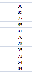
Based upon a range of values you can show the Red, Yellow or Green indicators in the cell. To create Traffic light lets take this sample data

Step 1
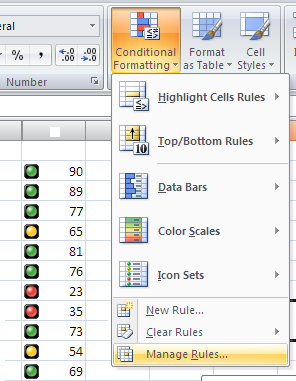
Select the data and click on the Conditional Formatting drop down from the Styles group of the Home tab

Step 2
Select Icon Sets and then 3 Traffic Lights

If you want to change the conditions, select Manage Rule from the Conditional Formatting drop down.

Select the rule then click on Edit Rule. Change the conditions then click on Ok

You can also check the Show Icon only check box to see only the lights and not the data.